
updated 2000.03.30
Author Arpad Buermen
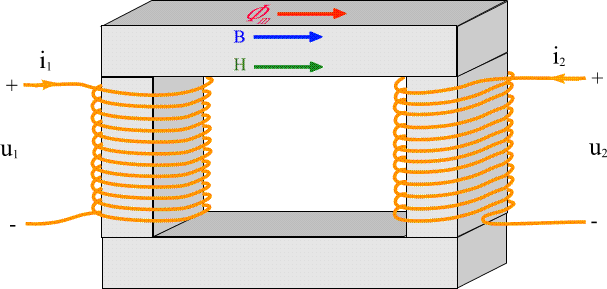
Modelling and Simulation of a Non-linear Transformer
Abstract: every device not found in the basic SPICE library must
be modelled using the elements from the library. A transformer is no exception.
Sure, there are some devices present in the basic SPICE library that can
be used directly to model a transformer (coupled inductances combined with
resistors provide a quite useful model). Unfortunately the simple coupled-inductances
model is appropriate only for linear analysis since it models the characteristics
of a linear transformer - a non-existent ideal of the real transformer that
can be used only when the core is well below saturation. In many specific
simulations of a circuit including a transformer the non-linear model must
be used; e.g. transient responses to power surges, power-on transient response,
etc.
When building a model the main issue is what to put in and what to
neglect. In case the care for details is exaggerated, the model is too
complex and the simulation takes long time even on state of the art hardware
with results just slightly more accurate than those obtained with a less
complex model. On the other hand excess simplification makes things even
worse since the results are inaccurate and in some cases SPICE algorithms
are unable to reach convergence.
A simple model of a non-linear transformer is presented below. The
model is then used to obtain the power-on transient response of a circuit
consisting of a transformer and various loads.
Basic info:
- Core:
- relative permitivity below the point of saturation ur = 3980
- relative permitivity above the point of saturation ur' = 180
- vacuum permitivity u0 = 4*PI*10-7 Vs/Am
- point of transition between linear operation and saturation - Hk = 200A/m, Bk = 1T
- average cross-section area of the core A = 2*10-4 m2
- average length of a line of force lsr = 0,2m
- Coils:
- primary coil windings N1 = 4470, N1*A = 0,894m2
- secondary coil windings N2 = 570, N2*A = 0,144m2
- primary coil resistance R1 = 300ohm
- secondary coil resistance R2 = 5ohm
- primary coil to ground resistance 1Gohm
- secondary coil to ground resistance 1Gohm
- The latter two resistances are necessary to define the potential of
the primary and secondary coil since SPICE doesn't allow floating circuits.
Modelling the core
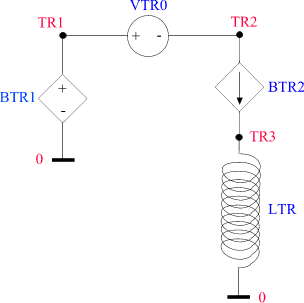
Since SPICE works with voltages and currents, equivalents must be chosen for magnetic flux density and magnetic field. Let the current be the equivalent of the magnetic flux density and the voltage the equivalent of the magnetic field. The basic idea is to build a circuit excited with voltage which is the equivalent of magnetic field (H). The response is the current which is the equivalent of magnetic flux density (B). Since magnetic field in the core depends on primary and secundary current, two linear current controlled voltage sources connected in series can model the relation between the coil currents and the magnetic field in the core:
- H = (N1 * i1 + N2 * i2)
/ lsr
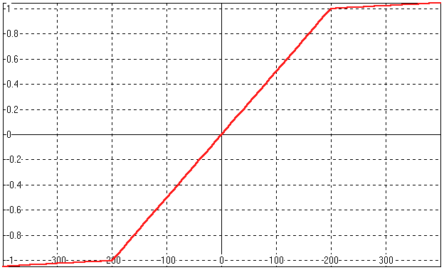
To model the non-linear B(H) response a non-linear voltage controlled current source BTR2 controlled with the TR1 node voltage is used.. The non-linear characteristic used in the model consists of three linear segments - one for linear operation (-Hk to Hk) and two for saturation (below -Hk and above Hk).
- B = u0 ( ur * H + (ur' - ur)
* ((H - Hk) * u(H - Hk) + (H + Hk) * u(
-(H + Hk)))
As mentioned before the loop current is the equivalent of the magnetic flux density (B). To model the interaction between the magnetic field in the core and the voltage induced in the primary and the secondary coil the first order derivative of magnetic flux density (dB/dt) must be available. It can be obtained by running the current generated by BTR2 through a 1H inductance. Thus node TR3 provides us with voltage equivalent of dB/dt.
Independent voltage source VTR0 is used to obtain the current which is the equivalent of magnetic flux density (B). Magnetic field can be obtained as the TR1 node voltage.
The above discussion gives the following model of the core:
BTR1 TR1 0 V=(4470*i(VTR1)+570*i(VTR2))/.20
VTR0 TR1 TR2 0V
BTR2 TR2 TR3
  + I=(3980*V(TR1)+
  + (180-3980)*((V(TR1)-200)*u( V(TR1)-200 )+
  + (V(TR1)+200)*u(-(V(TR1)+200))))
  + *1.256637e-6
LTR TR3 0 1H
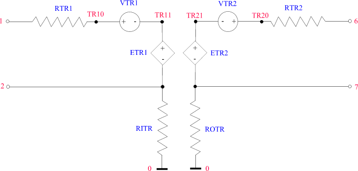
- Primary coil is modelled with a coil resistance RTR1, an independent
0V voltage source VTR1 used to obtain the primary coil current and
a voltage controlled voltage source ETR1 modelling induced voltage. The
latter is obtained using the following equation:
- Ui1 = N1 * A * dB/dt
The same goes for the secondary coil. The following equation is used to determine the induced voltage:
- Ui2 = N2 * A * dB/dt
Primary coil model:
RTR1 1 TR10 300ohm
VTR1 TR10 TR11 0V
ETR1 TR11 2 TR3 0 0.894
RITR 2 0 1Gohm
Secondary coil model:
RTR2 6 TR20 5ohm
VTR2 TR20 TR21 0V
ETR2 TR21 7 TR3 0 0.114
ROTR 7 0 1Gohm
Examples
-
 Open circuit secondary coil
 -
20ohm load on the secondary coil
-
A rectifier with 20ohm load, power-on transient
response
-
A rectifier with 20ohm load, steady state response
Conclusion
A non-linear transformer can be efficiently modelled using a simple circuit. Since the model developed above is so simple, the analysis is quick. It poses no problem to incorporate a more complex non-linear core B(H) characteristic since a non-linear voltage controlled current source was used providing a wide variety of functions (exp, sin, cos, th, etc.) for describing a curve.
In the next stage of the development modelling of hysteresis, imperfect magnetic coupling of coils and eddy current effects in the core should be considered.
The author is aware of his imperfect English. All suggestions concerning grammar and spelling are welcome.