updated 2000.11.30
Author Janez Puhan
Delay Lines
The circuit
If a large number of simple lag networks are connected in cascade, the resulting transfer function will approach that of a dead period lag. An impulse injected into the input terminals will appear at the output with a delay time, T. As a practical example, series inductances and shunt capacitances are distributed uniformly to simulate a coaxial or two wire line in the next two circuits.
An infinite number of discrete elements, n, with infinitely small size, has a transfer function of
Loss Free Delay Line

The input file
discontinuous loss free delay line

.control
tran 0.5ns 100ns
plot v(1)+2 v(3)*10+1 v(4)*10 v(5)*10-1 v(6)*10-2 xlabel t[s]
  + ylabel 'v(1) v(3) v(4) v(5) v(6) [V]' title 'TRAN analysis'
.endc

v1 1 0 dc 0 pulse 0 1 0 0 0 0.5ns 1s

r1 1 2 320
r2 6 0 320

x1 2 3 loss_free_line
x2 3 4 loss_free_line
x3 4 5 loss_free_line
x4 5 6 loss_free_line

.subckt loss_free_line 1 8
l1 1 2 0.5uH
l2 2 3 1uH
l3 3 4 1uH
l4 4 5 1uH
l5 5 6 1uH
l6 6 7 1uH
l7 7 8 0.5uH

c1 2 0 10pF
c2 3 0 10pF
c3 4 0 10pF
c4 5 0 10pF
c5 6 0 10pF
c6 7 0 10pF
.ends

.end
The results

Lossy Delay Line

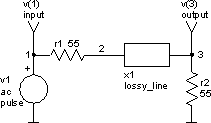
The input file
discontinuous lossy delay line

.control
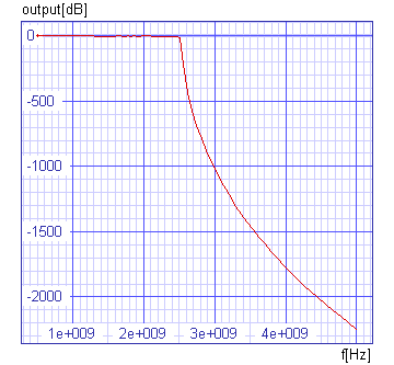
ac dec 100 0.5gHz 5gHz
plot vdb(3) linear xlabel f[Hz] ylabel output[dB] title 'AC analysis'
tran 0.1ns 20ns
plot v(1)/2+1.5 v(3) xlabel t[s] ylabel 'input output [V]' title 'TRAN analysis'
.endc

v1 1 0 dc 0 ac 2 pulse 0 2 1ns 0 0 4ns 1us

r1 1 2 55
r2 3 0 55

x1 2 3 lossy_line

.subckt lossy_line 1 11
x1 1 2 lossy_line1
x2 2 3 lossy_line1
x3 3 4 lossy_line1
x4 4 5 lossy_line1
x5 5 6 lossy_line1
x6 6 7 lossy_line1
x7 7 8 lossy_line1
x8 8 9 lossy_line1
x9 9 10 lossy_line1
x10 10 11 lossy_line1
.ends

.subckt lossy_line1 1 11
x1 1 2 rlcg
x2 2 3 rlcg
x3 3 4 rlcg
x4 4 5 rlcg
x5 5 6 rlcg
x6 6 7 rlcg
x7 7 8 rlcg
x8 8 9 rlcg
x9 9 10 rlcg
x10 10 11 rlcg
.ends

.subckt rlcg 1 3
r1 2 3 0.04
r2 3 0 750k

l1 1 2 6.88nH

c1 3 0 2.27pF
.ends

.end
The results

